Author Archives: admin

WHR Crosswalk for Sonoma Veg Map

California Wildlife Habitat Relations (CWHR) is a habitat classification system developed by the California Department of Fish and Wildlife.  The system classifies the California landscape into 59 wildlife habitats.  The system associates each of 712 wildlife species to the wildlife habitats where the species occurs.  Using information from the Manual of California Vegetation, Volume 2, and the CWHR Habitat Classification Rules, we developed a crosswalk from the 82 fine scale map classes in the Sonoma Veg Map to their respective WHR habitat types.  You can download the crosswalk as an MS Excel file here:  https://sonomaopenspace.egnyte.com/dl/IVMaWwISME

Hopefully this crosswalk is useful to wildlife managers in Sonoma County!  Please let us know if you have suggested revisions to the crosswalk.

1942 Imagery and Historic Photo Viewer Updated

Fearing a west coast invasion during World War II, the U.S. Department of War collected airphotographs of all of Sonoma County in 1942.  These photos are the earliest complete image of Sonoma County. The photos were collected on film and printed as thousands of hard copy (9" x 9") photos. Two complete hard copies remain - one at the University of California Berkeley and the other at Draftech in Santa Rosa.

Through grants from the Sonoma County Water Agency and the Sonoma County Agricultural Preservation and Open Space District, the San Francisco Estuary Institute (SFEI) has digitized, georeferenced, and mosaiced a subset of these 9x9 hard copy photos.  The original batch, completed in 2014, covered the Santa Rosa Plain.  In 2016, the Dry Creek Valley was added to the historic mosaic of photographs.  At the tail end of 2017, SFEI made the latest batch available, extending the historic air photo mosaic down to the Marin County line.  This dataset is useful for all manner of historical analysis such as understanding changes in land use and population, and tracking changes in vegetation and habitat over time.

The data is available as a tile service (search ArcGIS.com for 'Sonoma County 1942'), as a  tif file for download and use in GIS software, and in a historic photo viewer titled 'Central Sonoma County - Then and Now.'


Fires

Since the fires burned, we have been working on curating spatial data related to the fires. We are providing a roundup of post-fire datasets, articles, and resources to aid in fire response, assessment, and study. This work is part of an integrated watershed effort led by the Ag and Open and Space District in collaboration with the Sonoma County Water Agency, the Sonoma County Information Systems Department, NOAA, the Regional Water Board, Sonoma RCD, and a multitude of land managers and conservation groups.

See the data downloads page and look for '2017 fire data products' for links to post-fire imagery, canopy damage maps, and ladder fuel products.

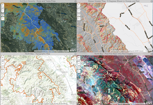
Soil Burn Severity Data

Soil burn severity data was produced by the United States Forest Service for the Nuns and Tubbs fires.  These data were produced in a two step process that included satellite image analysis of Worldview, Sentinel, and Spot data followed by field validation.  We will monitor agency web sites and update links and services as needed.

Soil Burn Severity 4-Pane Viewer
Soil Burn Severity Service
Soil Burn Severity Spatial Data & Maps (from CA Department of Conservation)

Soil Burn Severity 4-Panel Viewer


Debris Flow Likelihood Data

Debris flow likelihood data was produced by USGS.  The USGS approach uses empirical models that estimate likehood and volume of post-fire debris flows.  The models are based on "historical debris-flow occurrence and magnitude data, rainfall storm conditions, terrain and soils information, and burn severity data" (more on methods here).  We have published some of the data as services - specifically the likelihood of landslides (by stream segment and by basin) after a 6mm, 15-minute rainfall event.  We will monitor the USGS web site and update links and services as needed.

Landslide Likelihood 4-Pane Viewer
Landslide Likelihood Feature Service (Basins)
Landslide Likelihood Feature Service (Stream Segments)
Landslide Likelihood Data Download (download the full suite of debris-flow probability and volume data from USGS)

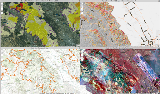
Debris Flow Likelihood 4-Panel Viewer


Fire History

The State of California (Calfire) maintains current and historic spatial data for California wildfires.  The spatial data, which contains perimeters of fires going back to the 1800s, is distributed and maintained by Calfire's Fire and Resource Assessment Program (FRAP).   The layer contains fire perimeters as polygons, along with associated information including fire name, start date, date of containment, cause of the fire, and more.  Calfire's spatial dataset is publicly available here.

Using Calfire's data, the Sonoma Land Trust developed a web mapping application that illustrates the history of fire in the region since the middle of the last century.  The tool lets you 'slide through time' to view fire activity.  The application also includes the perimeters of the Tubbs, Nunns, and Pocket fires.

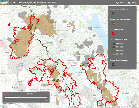
Sonoma Land Trust's Fire History Web Mapping Application


Imagery

Use the links below to access fire-related image datasets. Note that burned areas and living vegetation are most easily visible in color infrared (CIR) imagery.

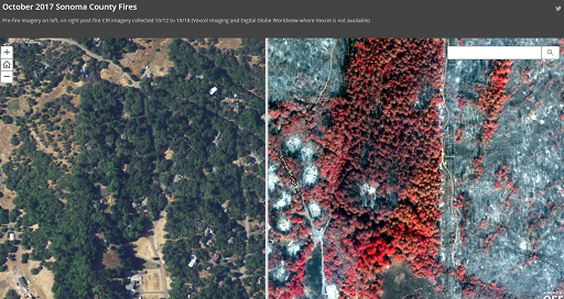
Viewer to Compare Pre and Post Fire Imagery

Watershed Emergency Response Team Reports (WERTS)
CalFire published WERTs for each North Bay fire in November 2017. These reports provide an overview of the fire and context about burned area geology, soil, and hydrology. The WERTs focus on burned areas especially at risk of post-fire debris flows and erosion. Download the WERTs at the links below:

[table "" not found /]

Other Fire GIS Data Resources


Fine-Scale Vegetation and Habitat Map Now Available!

We are thrilled to announce that the countywide vegetation and habitat map is complete and available for download. The Vegetation and Habitat map provides a fine-scale representation of natural vegetation in Sonoma County. The map has 212,391 polygons countywide, and represents 83 different vegetation communities and land cover types. The map was created using a combination of field work, aerial photo interpretation, and computer-based modeling and machine learning. The map is based on a vegetation key developed by the California Department of Fish and Wildlife and the California Native Plant Society for the Sonoma Veg Map Program.

Sonoma County Fine-Scale Vegetation and Habitat Map

The Fine-Scale Vegetation and Habitat map is the culmination of several years of hard work by a team led by the Sonoma County Agricultural Preservation and Open Space District and the Sonoma County Water Agency.

In the coming months, the Sonoma Veg Map team will complete an accuracy assessment for the Fine-Scale Vegetation and Habitat map. The accuracy assessment will include user's and producer's evaluation of accuracy for the more common fine scale map classes, as well as overall map accuracy. After the accuracy assessment is completed, it will be published along with a final report and methods document for the Fine-Scale Vegetation and Habitat map.

The Fine-Scale Vegetation and Habitat map is available as watershed downloads and countywide downloads in various formats from http://sonomavegmap.org/data-downloads. We have also produced a series of poster-sized vegetation and habitat PDF maps.  Also, check out this product datasheet, which provides details about the vegetation and habitat map.

Along with the vegetation map, there are a number of other related fine-scale map products that are now available for download.   For more information, check out our Spring, 2017 newsletter.

Historic 'Soil-Veg' Maps Available for Northern Sonoma Cty.

We are very excited to announce the availability of a set of historic vegetation maps for the northern portion of Sonoma County.  The maps are the 'Soil-Veg' maps published in collaboration by California's Department of Forestry (now CalFire), the University of California, and the U.S.D.A. Forest Service between 1947 and 1980.  The maps contain detailed information about soils, dominant vegetation (listed by species in descending order of dominance), and timber site quality index.

If you use these maps, please remember that they are very old and reflect the state of landscape between 40 and 70 years ago (date varies by 7.5 minute U.S.G.S. quad - see index map below).  Also bear in mind that the maps were created at a small scale (1:31,680) and with far less advanced methods than those used in today's digital age.

Kass Green and Gene Forsburg (part of the Sonoma Veg Map team) were familiar with these maps and - when they realized the maps had probably never been scanned and georeferenced - asked Dr. Maggi Kelly (a Sonoma Veg Map advisor) at UC Berkeley's Geospatial Innovation Facility (GIF) about them.  Dr. Kelly tracked down the old maps, finding them at the Biosciences & Natural Resources Library and the Earth Sciences and Map Library.  Through a generous gift from Kass and Gene to the GIF, UC Berkeley scanned and georeferenced the Soil-Veg map quads for Sonoma County. Thanks to these U.C. Berkeley Libraries for taking good care of the maps for all of these years so that we can share them with you today!

Even though the 'Soil-Veg' maps are small-scale and old, they provide a key to species distribution for our team in areas where access is impossible. The 20th century veg. mappers were able to access broad areas of the county and used field visits in conjunction with photo interpretation of stereo pairs of aerial photography to make the maps.

We are very excited because we know these maps have been helpful to us, and we think that they will be useful to others, especially those interested in the state of the landscape in the second half of the last century.

The maps are packed with information.  The graphic below shows part of a polygon and provides a rudimentary decoding of the information on the maps. Refer to the list of resources at the end of this post for more detailed information about the maps.

Explanation of Soil-Veg Map Polygon Labels

Explanation of Soil-Veg Map Polygon Labels

The 'Soil-Veg' maps were created by 7.5 minute U.S.G.S. quad. The GIF scanned and georeferenced each of the individual quads (see map below) and then mosaiced them without their collars into a single TIF image. The TIF is available for download, and the mosaic has also been published as a tile service (see below for links).

Area of Availability Soil-Veg Maps

Soil-Veg Map Availability and Dates When Mapping Occurred for Each Area

Here's how to get the 'Soil-Veg' maps and related information:

  • Check out this story map!
  • Work with the maps in ArcMap by downloading this TIF image of the maps (2 GBs)
  • Download the list of species abbreviations (you'll need this!)
  • Download an legend/user's guide (for one of the individual Sonoma County quads)
  • Download a product description that includes info about the 'Soil-Veg' maps
  • Use the quad index grid for the 'Soil-Veg' maps, which includes in its attributes the years of field work and mapping for each U.S.G.S. quad (these are the quad polygons shown in the map above)
  • View this blog post from Dr. Kelly, which includes estimated horizontal error for each scanned and georeferenced 'Soil-Veg' map quad

Hydrologic Data Products Now Available

We're excited to announce the release of a suite of hydrologic data products.

Clockwise from upper left - flow direction, flow accumulation, stream centerlines, and orthophotos (image by Quantum Spatial)

These Sonoma County hydrologic data products were produced in fall 2015 and winter 2016 from the countywide 2013 LiDAR data. The hydrologic products include a set of vector deliverables and a set of raster deliverables. Vector products include stream centerlines, confluence points, hydroenforcement burn locations, and watersheds. Raster products include flow direction, flow accumulation, and a hydroenforced bare earth digital elevation model (DEM). Hydroenforcement of a DEM imparts the true elevations of culverts, pipelines, and other buried passages for water into a Digital Elevation Model, creating a DEM suitable for modeling the flow of surface water.

The extent of the deliverables is all of Sonoma County, the Lake Sonoma watershed in Mendocino County, and the Lake Mendocino area.

These hydrologic datasets are a mostly-automated first step in the eventual development of a 'localized' or 'LiDAR enhanced' National Hydrography Dataset (NHD). They are suitable for landscape level planning and hydrologic modeling. These data products do not contain a guarantee of accuracy or precision and – without site specific validation and/or refinement – should not be relied upon for engineering level or very fine scale decision making.

The hydrologic data products were produced by Quantum Spatial. Read Quantum Spatial's Sonoma County Hydroenforcement Technical Data Report.

The individual hydrologic data products are described briefly below.

Vector Hydrologic Products (available here as a file geodatabase)

  • Stream Centerlines – Centerlines of streams in Sonoma County. An area of flow concentration is considered a stream if its flow accumulation (upstream catchment area) exceeds 5 acres and a clearly defined channel exists. Where possible, stream centerline names (GNIS_Name) are consistent with the NHD.
  • Hydroenforcement Burn Locations - Line features that represent locations where hydroenforcement occurred.
  • Confluence Points – Points that represent stream intersections (confluences).
  • Watersheds (HUC2 through HUC14) – Watershed boundaries for nested hydrologic units from HUC 2 (region) to HUC 14 (sub-watershed). Where possible, watershed names are consistent with the NHD. Watershed mapping conventions follow those for NHD's Watershed Boundary Dataset (http://nhd.usgs.gov/wbd.html).

Raster Hydrologic Products (1-meter resolution - available as watershed downloads)

  • Hydroenforced Digital Elevation Model – The Hydroenforced DEM is the LiDAR derived (2013) bare earth DEM with contours, pipelines and other buried passages to water 'burned in', so that the DEM correctly models surface water flow.
  • Flow Direction Rasters – Values in a flow direction raster represent one of eight directions (pixel values range from 1 to 8); No Data represents areas where there is no flow off of the pixel (sinks).
  • Flow Accumulation Rasters – Flow accumulation is a measure of upstream catchment area. Pixel values in a flow accumulation raster represent the cumulative number of upstream pixels (in other words, the count of pixels that contribute flow to a given pixel).

The webmap below shows the HUC 12 watersheds and the stream centerlines.

Countywide Lifeform and Cropland Datasets Available

Draft Lifeform Map: We are excited to announce that a draft lifeform map is complete and available for download. It will serve as the foundation for the more detailed vegetation and habitat map to come. This 18-class map was developed using a combination of automated, software-based processes and the input of GIS and vegetation analysts. Follow this link to learn more about the lifeform mapping methods.

The draft lifeform map (see interactive webmap below) will be refined in 2016 based on the field work and additional manual editing associated with producing the full 62-class fine-scale vegetation and habitat map due out in late 2016. Until then, the lifeform map can serve as an excellent reference map with high accuracy (read the accuracy assessment at the end of the product datasheet). Please reference this as a draft data product in your maps, analysis, and derivative products.

Sonoma County Draft Lifeform Map
View larger map

Final Croplands: The Sonoma County Croplands map, which we released as a draft product in the spring, has been updated and finalized. The croplands data provides a countywide fine-scale polygon map of perennial croplands, annual croplands, nurseries, orchards/groves, vineyards, and other crops. The croplands were mapped by image analysts using aerial photographs as ground reference and - as for the lifeform dataset above - this layer represents the state of the landscape in 2013.

The croplands data combines many years of quality mapping work by many hands - including Circuit Rider Productions, Dr. Adina Merenlender's Lab (UC Berkeley), the Sonoma County Agricultural Preservation and Open Space District, and the Sonoma County Water Agency - into one seamless dataset. During the past year, the Sonoma Veg Map mapping team has further improved and standardized the data, adding hundreds of new polygons and refining the majority of existing ones.

The lifeform and croplands are available as services from ArcGIS.com and as GIS data downloads (shapefiles and geodatabases). To download the data, go to the data downloads page on our web site. Also, download the product datasheets for the croplands and lifeform datasets. For an immediate look at the lifeform map, check out this webmap.

Water Agency Uses LiDAR Data to Help Restore Riparian Forests

As part of its Streamside Maintenance Program (SMP), The Sonoma County Water Agency has been using the 2013 Countywide LiDAR data to help manage vegetation within 175 miles of stream channels they are responsible to maintain for flood control. Each summer, the Water Agency works to remove undesirable vegetation and prune riparian trees. The goal of this work is to transition these channels into waterways that not only provide flood protection, but also provide good riparian habitat and water quality. With this type of management continuing over time, channel vegetation will grow and mature, with alders and other trees stretching their branches over the creek, cooling the water and shading out non-native blackberry and other less desirable species that reduce the water-carrying capacity of the creek.

To help identify where to promote the growth of desirable riparian trees, the water agency needs accurate maps of tree canopy density, or the portion of the ground overhung by trees. Tree canopy density was produced countywide from the 2013 LiDAR point cloud for Sonoma Veg Map. Before LiDAR, canopy density mapping required manual aerial photo interpretation – a laborious and costly effort. The LiDAR-derived canopy density data was used by Water Agency GIS staff to efficiently create maps of tree canopy density by channel reach (see map below). Water Agency staff are using these maps to target future vegetation management activities to where they are needed most. By comparing the 2013 LiDAR derived density maps to older canopy density maps, Water Agency staff can also evaluate the benefits of past vegetation management activities on riparian habitat.

For more information, contact Keenan Foster.

An Example of the Sonoma County Water Agency's LiDAR Derived Canopy Density Maps

An Example of the Sonoma County Water Agency's LiDAR Derived Canopy Density Maps

LiDAR Data Improves County's Road Centerline Maps

Explore this Story Map to See How the LiDAR Hillshade Helps with Road Mapping

Explore this Story Map to See How the LiDAR Hillshade Helps with Road Mapping

Sonoma County has benefited from the NASA-funded 2013 LiDAR data in many ways. One recent example is the County's GIS Group's use of the LiDAR-derived hillshade for improving road centerline delineations. Road centerlines have many uses: they form the base reference layer for navigation, they are critical for the county's emergency response services, they serve as a key input for natural resource conservation planning, and they are integral to the operations of county and state agencies that maintain the county's roads and transportation network.

Until now, road centerline delineation relied solely on orthophoto interpretation and occasionally GPS data collection, which can be costly. Since dense tree canopy sometimes covers roads, which renders them invisible on orthophotographs, the road centerline data is prone to accuracy problems. Additionally, GPS error increases under tree canopy, which can lead to accuracy problems even for road centerlines mapped with GPS.

Now with the LiDAR bare earth hillshade, which provides a three dimensional depiction of the ground even under canopy, we have a way to significantly improve road centerline accuracy. The image below shows a heavily forested section of Fort Ross Road (the road is shown in dotted yellow). The top pane shows the 2011 orthophotography. Because of the high tree density in this area, locating the road with the photo would be guesswork. However, in the bare earth hillshade (bottom pane), the road is clearly visible in darker tones than the surrounding landscape.

Fort Ross Road (dotted yellow) - Orthos Above; Bare Earth Hillshade Below

Fort Ross Road (dotted yellow) - Orthos Above; Bare Earth Hillshade Below

Check out this story map to see explore some areas that illustrate the benefits of using the LiDAR hillshade for mapping road centerlines.

Using the LiDAR bare earth hillshade, County of Sonoma Information Services Department (ISD) GIS Group has made significant strides in correcting misaligned centerlines under canopy in the countywide roads dataset – the result is a greatly improved and much more reliable roads layer. The Sonoma Veg Map team is using similar techniques to contribute improvements to the roads layer for use in impervious surface mapping.

Sonoma LiDAR Data Assists in Road Design

As the first in an occasional series on our blog, we're posting about how folks are using the 2013 SonomaVegMap LiDAR data. Mark Wein, Civil Engineer for Sonoma County's Department of Transportation and Public Works, uses the LiDAR point cloud to help when designing new roads and bridges. Mark uses Autodesk products to create triangulated area networks (TINS) from the point cloud. The software provides Mark with advanced point cloud filtering options that give him the ability to create his own customized ground surface TINs for a project area.

Mark brings the resulting ground surface TINs into AutoCAD (Civil 3D 2013) to create a preliminary design. Mark says "I really enjoy how fast it is to take the point cloud, create a TIN surface, pull the surface into Infraworks, add in the SonomaVegMap orthos and buildings footprints, and layout a quick road design."

The resulting road designs and TIN surfaces help Mark and other TPW staff to design new road infrastructure and to perform watershed and water drop analysis. Thanks very much Mark for sharing your work with SonomaVegMap!

Planned Fulton Creek Bridge Design from 2013 SonomaVegMap LiDAR & Orthos  (courtesy Mark Wein)

Planned Fulton Creek Bridge Design from 2013 SonomaVegMap LiDAR & Orthos (courtesy Mark Wein)