Category Archives: Uncategorized

Kincade Fire

Thanks to the firefighters out there doing incredible work. We just wanted to post a few resources related to the Kincade Fire.

Webmap showing Kincade footprint (updated daily), MODIS/VIIRS hotspots (updated several times daily), Tubbs/Nuns/Pocket fooprints, and weather data.

Sonoma County Department of Emergency Services webmap showing evacuation areas, road closures, and shelters.

Daily fire perimeter as a shapefile (Geomac)

Relativized Burn Ratio-Kincade Fire (Dr. Matthew Clark)

Sonoma County 5-meter Resolution Fuel Model

CNPS Fire Recovery Guide

2017 North Bay Fires Story Map

WHR Crosswalk for Sonoma Veg Map

California Wildlife Habitat Relations (CWHR) is a habitat classification system developed by the California Department of Fish and Wildlife.  The system classifies the California landscape into 59 wildlife habitats.  The system associates each of 712 wildlife species to the wildlife habitats where the species occurs.  Using information from the Manual of California Vegetation, Volume 2, and the CWHR Habitat Classification Rules, we developed a crosswalk from the 82 fine scale map classes in the Sonoma Veg Map to their respective WHR habitat types.  You can download the crosswalk as an MS Excel file here:  https://sonomaopenspace.egnyte.com/dl/IVMaWwISME

Hopefully this crosswalk is useful to wildlife managers in Sonoma County!  Please let us know if you have suggested revisions to the crosswalk.

1942 Imagery and Historic Photo Viewer Updated

Fearing a west coast invasion during World War II, the U.S. Department of War collected airphotographs of all of Sonoma County in 1942.  These photos are the earliest complete image of Sonoma County. The photos were collected on film and printed as thousands of hard copy (9" x 9") photos. Two complete hard copies remain - one at the University of California Berkeley and the other at Draftech in Santa Rosa.

Through grants from the Sonoma County Water Agency and the Sonoma County Agricultural Preservation and Open Space District, the San Francisco Estuary Institute (SFEI) has digitized, georeferenced, and mosaiced a subset of these 9x9 hard copy photos.  The original batch, completed in 2014, covered the Santa Rosa Plain.  In 2016, the Dry Creek Valley was added to the historic mosaic of photographs.  At the tail end of 2017, SFEI made the latest batch available, extending the historic air photo mosaic down to the Marin County line.  This dataset is useful for all manner of historical analysis such as understanding changes in land use and population, and tracking changes in vegetation and habitat over time.

The data is available as a tile service (search ArcGIS.com for 'Sonoma County 1942'), as a  tif file for download and use in GIS software, and in a historic photo viewer titled 'Central Sonoma County - Then and Now.'


Countywide Lifeform and Cropland Datasets Available

Draft Lifeform Map: We are excited to announce that a draft lifeform map is complete and available for download. It will serve as the foundation for the more detailed vegetation and habitat map to come. This 18-class map was developed using a combination of automated, software-based processes and the input of GIS and vegetation analysts. Follow this link to learn more about the lifeform mapping methods.

The draft lifeform map (see interactive webmap below) will be refined in 2016 based on the field work and additional manual editing associated with producing the full 62-class fine-scale vegetation and habitat map due out in late 2016. Until then, the lifeform map can serve as an excellent reference map with high accuracy (read the accuracy assessment at the end of the product datasheet). Please reference this as a draft data product in your maps, analysis, and derivative products.

Sonoma County Draft Lifeform Map
View larger map

Final Croplands: The Sonoma County Croplands map, which we released as a draft product in the spring, has been updated and finalized. The croplands data provides a countywide fine-scale polygon map of perennial croplands, annual croplands, nurseries, orchards/groves, vineyards, and other crops. The croplands were mapped by image analysts using aerial photographs as ground reference and - as for the lifeform dataset above - this layer represents the state of the landscape in 2013.

The croplands data combines many years of quality mapping work by many hands - including Circuit Rider Productions, Dr. Adina Merenlender's Lab (UC Berkeley), the Sonoma County Agricultural Preservation and Open Space District, and the Sonoma County Water Agency - into one seamless dataset. During the past year, the Sonoma Veg Map mapping team has further improved and standardized the data, adding hundreds of new polygons and refining the majority of existing ones.

The lifeform and croplands are available as services from ArcGIS.com and as GIS data downloads (shapefiles and geodatabases). To download the data, go to the data downloads page on our web site. Also, download the product datasheets for the croplands and lifeform datasets. For an immediate look at the lifeform map, check out this webmap.

Water Agency Uses LiDAR Data to Help Restore Riparian Forests

As part of its Streamside Maintenance Program (SMP), The Sonoma County Water Agency has been using the 2013 Countywide LiDAR data to help manage vegetation within 175 miles of stream channels they are responsible to maintain for flood control. Each summer, the Water Agency works to remove undesirable vegetation and prune riparian trees. The goal of this work is to transition these channels into waterways that not only provide flood protection, but also provide good riparian habitat and water quality. With this type of management continuing over time, channel vegetation will grow and mature, with alders and other trees stretching their branches over the creek, cooling the water and shading out non-native blackberry and other less desirable species that reduce the water-carrying capacity of the creek.

To help identify where to promote the growth of desirable riparian trees, the water agency needs accurate maps of tree canopy density, or the portion of the ground overhung by trees. Tree canopy density was produced countywide from the 2013 LiDAR point cloud for Sonoma Veg Map. Before LiDAR, canopy density mapping required manual aerial photo interpretation – a laborious and costly effort. The LiDAR-derived canopy density data was used by Water Agency GIS staff to efficiently create maps of tree canopy density by channel reach (see map below). Water Agency staff are using these maps to target future vegetation management activities to where they are needed most. By comparing the 2013 LiDAR derived density maps to older canopy density maps, Water Agency staff can also evaluate the benefits of past vegetation management activities on riparian habitat.

For more information, contact Keenan Foster.

An Example of the Sonoma County Water Agency's LiDAR Derived Canopy Density Maps

An Example of the Sonoma County Water Agency's LiDAR Derived Canopy Density Maps

LiDAR Data Improves County's Road Centerline Maps

Explore this Story Map to See How the LiDAR Hillshade Helps with Road Mapping

Explore this Story Map to See How the LiDAR Hillshade Helps with Road Mapping

Sonoma County has benefited from the NASA-funded 2013 LiDAR data in many ways. One recent example is the County's GIS Group's use of the LiDAR-derived hillshade for improving road centerline delineations. Road centerlines have many uses: they form the base reference layer for navigation, they are critical for the county's emergency response services, they serve as a key input for natural resource conservation planning, and they are integral to the operations of county and state agencies that maintain the county's roads and transportation network.

Until now, road centerline delineation relied solely on orthophoto interpretation and occasionally GPS data collection, which can be costly. Since dense tree canopy sometimes covers roads, which renders them invisible on orthophotographs, the road centerline data is prone to accuracy problems. Additionally, GPS error increases under tree canopy, which can lead to accuracy problems even for road centerlines mapped with GPS.

Now with the LiDAR bare earth hillshade, which provides a three dimensional depiction of the ground even under canopy, we have a way to significantly improve road centerline accuracy. The image below shows a heavily forested section of Fort Ross Road (the road is shown in dotted yellow). The top pane shows the 2011 orthophotography. Because of the high tree density in this area, locating the road with the photo would be guesswork. However, in the bare earth hillshade (bottom pane), the road is clearly visible in darker tones than the surrounding landscape.

Fort Ross Road (dotted yellow) - Orthos Above; Bare Earth Hillshade Below

Fort Ross Road (dotted yellow) - Orthos Above; Bare Earth Hillshade Below

Check out this story map to see explore some areas that illustrate the benefits of using the LiDAR hillshade for mapping road centerlines.

Using the LiDAR bare earth hillshade, County of Sonoma Information Services Department (ISD) GIS Group has made significant strides in correcting misaligned centerlines under canopy in the countywide roads dataset – the result is a greatly improved and much more reliable roads layer. The Sonoma Veg Map team is using similar techniques to contribute improvements to the roads layer for use in impervious surface mapping.

Sonoma LiDAR Data Assists in Road Design

As the first in an occasional series on our blog, we're posting about how folks are using the 2013 SonomaVegMap LiDAR data. Mark Wein, Civil Engineer for Sonoma County's Department of Transportation and Public Works, uses the LiDAR point cloud to help when designing new roads and bridges. Mark uses Autodesk products to create triangulated area networks (TINS) from the point cloud. The software provides Mark with advanced point cloud filtering options that give him the ability to create his own customized ground surface TINs for a project area.

Mark brings the resulting ground surface TINs into AutoCAD (Civil 3D 2013) to create a preliminary design. Mark says "I really enjoy how fast it is to take the point cloud, create a TIN surface, pull the surface into Infraworks, add in the SonomaVegMap orthos and buildings footprints, and layout a quick road design."

The resulting road designs and TIN surfaces help Mark and other TPW staff to design new road infrastructure and to perform watershed and water drop analysis. Thanks very much Mark for sharing your work with SonomaVegMap!

Planned Fulton Creek Bridge Design from 2013 SonomaVegMap LiDAR & Orthos  (courtesy Mark Wein)

Planned Fulton Creek Bridge Design from 2013 SonomaVegMap LiDAR & Orthos (courtesy Mark Wein)

1942 Aerials of Sonoma County - Santa Rosa Plain

Fearing a west coast invasion during World War II, the U.S. Department of War collected airphotographs of all of Sonoma County in 1942.  These photos are the earliest complete image of Sonoma County. The photos were collected on film and printed as thousands of hard copy (9" x 9") photos. Two complete hard copies remain - one at the University of California Berkeley and the other at Draftech in Santa Rosa.

Through a grant from the Sonoma County Water Agency and the Sonoma County Agricultural Preservation and Open Space District, the San Francisco Estuary Institute (SFEI) has digitized, georeferenced, and mosaiced a subset of the photos - those that comprise the Santa Rosa Plain. This dataset is useful for all manner of historical analysis such as understanding changes in land use and population, and tracking changes in vegetation and habitat over time.

Check out the embedded map below (click here for the full version) to easily compare what things looked like in 1942 to what they look like today in the Santa Rosa Plain. Watch out - it's addicting! You can also download the air photography here (700 MB .img file).  If you want to use the photography as an ESRI image service, search ArcGIS.com for 'Sonoma County 1942'.

Click here for the full version

Overview of Vegetation Mapping Methods

The Sonoma County Vegetation and Habitat Mapping Program will use a state of the art mapping approach that combines on the ground field data collection with modern semi-automated mapping techniques. The semi-automated approach leverages the power of today's expert systems and machine learning algorithms to automate the mundane and laborious parts of vegetation mapping, such as delineating stand boundaries and labeling obvious features, saving valuable expert labor for the more subtle and difficult components of mapping.

Field Data Collection to Support Mapping
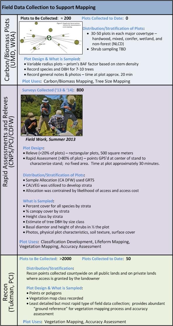
Field work is a critical component to any vegetation mapping project. As shown in Figure 1 (below), there are three types of field data that will be collected and utilized for vegetation mapping: carbon/biomass plots, rapid assessment and releve plots, and reconnaissance (recon). Variable radius plots will be collected using a prism to support the biomass and carbon mapping being conducted by Dr. Ralph Dubayah (University of Maryland) under a NASA Roses Grant. These plots will accurately measure living biomass across Sonoma County's woody habitats. The biomass measurements will be used by Dr. Dubayah's team to develop models that will be used to map woody biomass across all of Sonoma County.

Rapid assessment and releve plot collection will provide a base of very detailed species composition information across the county's habitats - these plots will be used to refine the rules and descriptions for Sonoma County's vegetation types, resulting in a classification (based on A Manual of California Vegetation), a dichotomous key, and type descriptions. The rapid assessment and releve plots - along with extensive field reconnaissance data - will be used for all phases of the vegetation mapping process, as well as for accuracy assessment. Sonoma Veg Map is lucky to be the beneficiary of an in-kind grant from the California Department of Fish and Wildlife's Vegetation Mapping and Classification Program (VegCAMP). VegCAMP, led by Dr. Todd Keeler-Wolf, has played and will continue to play an instrumental role in field data collection, plot data analysis, and classification development for Sonoma Veg Map.

Figure 1 - Field Data Collection
plots

Lifeform Mapping
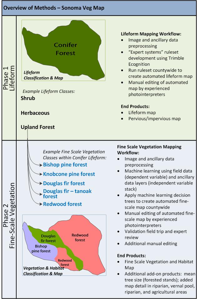
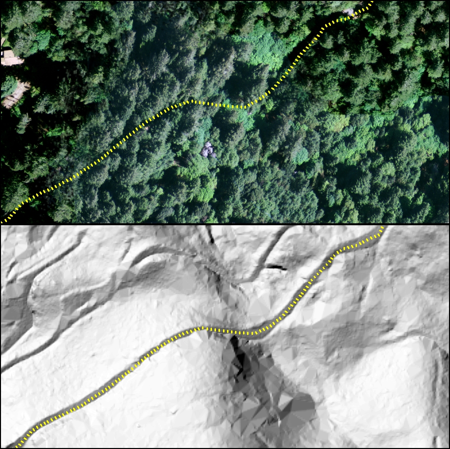
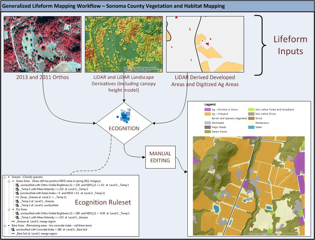
Mapping will occur in two phases: lifeform mapping and fine-scale vegetation mapping (see Figure 3 at the end of this post). The lifeform map serves as the foundation for the much more detailed fine-scale vegetation map. The lifeform map utilizes "expert systems" rulesets that are developed in Trimble Ecognition. These rulesets combine automated image segmentation (stand delineation) with object based image classification techniques. In contrast with machine learning approaches, expert systems rulesets are developed heuristically based on the knowledge of experienced image analysts.  Key data sets that will be used in the expert systems rulesets for lifeform include:  orthophotography ('11 and '13), the LiDAR derived Canopy Height Model (CHM), and other LiDAR derived landscape metrics. Figure 2 shows the lifeform mapping workflow.

After it is produced using Ecognition, the preliminary lifeform map product is manually edited by photointerpreters. Manual editing corrects errors where the automated methods produced incorrect results. Edits are made to correct two types of errors: 1) unsatisfactory polygon (stand) delineations and 2) incorrect polygon labels.

The lifeform map classifies the landscape into the following basic cover type classes:

  • Urban Window
  • Water
  • Barren & Sparsely Vegetated
  • Major Road
  • Developed
  • Orchard or Grove
  • Vineyard
  • Vineyard Replant
  • Annual Cropland
  • Perennial Agriculture
  • Irrigated Pasture
  • Intensively Managed Hayfield
  • Nursery or Ornamental Horticultural Area
  • Native Forest
  • Non-Native Forest
  • Shrub
  • Non-Native Shrub
  • Herbaceous

The impervious surface map, a separate Sonoma Veg Map product, will provide very detailed delineations of impervious surfaces, with a minimum mapping unit of 1000 square feet.  Impervious surfaces will be mapped using the following classes:

  • Buildings
  • Dirt and Gravel Roads
  • Paved Roads
  • Other Impervious

Figure 2 - Lifeform Mapping Workflow
Mapping Workflows - General

Fine-Scale Vegetation Mapping
The second phase of mapping refines the lifeform product into a fine-scale vegetation map. This process relies on machine learning algorithms which identify and exploit correlations between field surveyed vegetation and a "stack" of independent variables derived from ancillary geospatial data sets. The resulting machine-learning-based model is applied to the entire landscape, resulting in a preliminary fine-scale vegetation map.  Machine learning algorithms utilized for this process will include Classification and Regression Tree Analysis (CART) and Random Forests.  The independent variables used for this project will include the following:

  • Spectral bands and indices (means and stand deviations) derived from 2011 and 2013 orthophotography
  • Spectral bands and indices derived from multi-temporal Landsat imagery
  • Key spectral indices from AVIRIS (hyperspectral) - Thanks Dr. Matthew Clark for access to this data!
  • Canopy volume profiles derived from the LiDAR point cloud
  • LiDAR derived slope and aspect
  • LiDAR derived elevation
  • LiDAR derived landscape metrics
  • MODIS-derived fog/cloud frequency (thanks to Dr. Eric Waller for providing this data set!)
  • Shape indices that characterize stand shape, derived from Trimble Ecognition
  • Numerous layers from the California Basin Characterization Model (BCM), including average annual precipitation and climate water deficit
  • Horizontal distance from coastline

After it is produced the machine learning approach, the preliminary fine scale vegetation map product is manually edited by photointerpreters.  Manual editing corrects errors where the automated methods produced incorrect results. Edits are made to correct two types of errors: 1) unsatisfactory polygon (stand) delineations and 2) incorrect polygon labels. After an initial round of editing is complete, draft maps are reviewed by local experts and field crews are dispatched for a final round of map review. Based on input from local experts and notes from the final map review, the fine-scale vegetation map is manually edited one final time before delivery.

Figure 3 - Overview of Methods
methods

Welcome!

Welcome to the Sonoma County Vegetation and Habitat Mapping blog!  This blog will facilitate an ongoing discussion between the mapping team, the map's stakeholders, and end users of the maps.  We will also use this forum to make our community aware of program related events and milestones.